An official website of the United States government
Here’s how you know
Official websites use .gov A .gov website belongs to an official government organization in the United States.
Secure .gov websites use HTTPS A lock ( ) or https:// means you’ve safely connected to the .gov website. Share sensitive information only on official, secure websites.
Breeding ecology studies of boreal waders have been relatively scarce in North America. This paucity is due in part to boreal habitats being difficult to access, and boreal waders being widely dispersed and thus difficult to monitor. Between 2008 and 2014 we studied the nesting ecology of Whimbrels Numenius phaeopus hudsonicus in interior Alaska, a region characterized by an active wildfire regime. Our objectives were to (1) describe the nesting ecology of Whimbrels in tundra patches within the boreal forest, (2) assess the influence of habitat features at multiple scales on nest-site selection, and (3) characterize factors affecting nest survival. Whimbrels nested in the largest patches and exhibited a consistently compressed annual breeding schedule. We hypothesized that these Whimbrels would exhibit synchronous and clustered nesting, but observed synchronous nesting in only 2009 and 2011, and evidence of clustered nesting at just one study area in 2009, providing limited support for the hypothesis. Nests tended to be on hummocks and exhibited lateral concealment around the bowl, suggesting a trade-off between a greater view from the nest and concealment. However, our analysis failed to identify other important habitat features at scales from 1–400 m from the nest. Our best-supported nest survival model showed a strong difference between our two main study areas, but this difference remains largely unexplained. Given the increased frequency, severity, and extent of wildfires predicted under climate change climate change Climate change includes both global warming driven by human-induced emissions of greenhouse gases and the resulting large-scale shifts in weather patterns. Though there have been previous periods of climatic change, since the mid-20th century humans have had an unprecedented impact on Earth's climate system and caused change on a global scale.
Learn more about climate change scenarios, our study highlights the importance of monitoring the persistence of boreal tundra patches and the Whimbrels breeding therein.
INTRODUCTION
Whimbrels Numenius phaeopus breed throughout the Holarctic, mostly in treeless, open habitats (Cramp & Simmons 1983). The North American subspecies N. p. hudsonicus (AOU 1998) nests in two disjunct regions, one confined mostly to Alaska and W Canada (i.e., the proposed N. p. rufiventris; Engelmoer & Roselaar 1998), and the other around Hudson Bay, Canada (Skeel & Mallory 1996). In northern and western Alaska, Whimbrels are considered widespread, discontinuous breeders beyond the treeline (Gotthardt et al. 2013). Within interior Alaska and NW Canada, however, Whimbrels appear to breed primarily in tundra-like patches, either in contiguous stretches (e.g., subalpine) or interspersed among boreal forests (Sinclair et al. 2003, Gibson 2011, Gotthardt et al. 2013). This area is characterized by a boreal forest-tundra ecotone comprising a vast mosaic of postfire communities, including lichen-shrub tundra and lichen-spruce woodlands (Payette et al. 2001). Yet despite the limited extent of tundra here (Jorgenson & Meidinger 2015) compared to sites in W and N Alaska, 50% (perhaps 20,000) of the western population of North American Whimbrels are thought to breed within the boreal forest biome (Wells & Blancher 2011, Andres et al. 2012).
This biome is characterized by disturbance, with wildfires arguably the most important factor shaping habitats, both spatially (local) and temporally (annual to decadal; Kasischke et al. 2010). The boreal region, however, is increasingly threatened by disturbances related to a warming climate and these act on larger (landscape-level) and longer(decades to centuries) scales (Grosse et al. 2011). Advancing tree line (Lloyd 2005), wetland drying (Riordan et al. 2006, Roach 2011), peatland loss (Frolking et al. 2011), increased shrubification (Tape et al. 2006), and more active fire regimes (Kasischke & Turetsky 2006, Kasischke et al. 2010) are all hypothesized broad-based, long-term disturbances to this region that could further impact boreal tundra-like habitats in which Whimbrels currently breed.
In light of these predicted changes to boreal forest habitats, we studied the nesting ecology of Whimbrels breeding in interior Alaska, a region characterized by a continental climate and having an active wildfire regime (Kasischke et al. 2006). Indeed, this is the most comprehensive study of Whimbrels breeding in Alaska, and the first extensive breeding study of any boreal wader species in interior Alaska. We wanted to identify factors that may limit the distribution and nesting success of Whimbrels in their patchily distributed breeding habitats within the boreal forest biome. Our primary objective was to describe the nesting ecology of Whimbrels in tundra patches within the boreal forest, including metrics of phenology (arrival through hatch), nest density, and nest success. We also assessed habitat features at multiple spatial scales to determine their importance in the selection of nest sites (Jones & Robertson 2001, Bailey & Thompson 2007).
The Whimbrel is an aggressive attack-mobbing species that relies on early detection of predators (Skeel 1983, Skeel & Mallory 1996). We hypothesized that boreal breeding Whimbrels would nest synchronously and in clusters to enhance joint nest defense. Further, because the placement of nests for many open-nesting bird species (including waders; Götmark et al. 1995, van der Vliet et al. 2008, Gómez-Serrano & López-López 2014) may represent a trade-off between concealment (e.g., landform, complexity of vegetative cover) and providing the incubating bird a clear view of its surroundings, we hypothesized that Whimbrels would select nest sites that were elevated for view, yet still inconspicuous. We predicted that nesting earlier, nearer to conspecifics, and with fewer large obstacles (i.e., medium and tall shrubs, trees; Ballantyne & Nol 2011) to limit view from the nest, would increase Whimbrels’ nest survival. Finally, we measured habitat preferences to predict how Whimbrels might respond to more woody environments projected under future climates (Lloyd 2005, Tape et al. 2006).
METHODS
Study area
We studied the nesting biology of Whimbrels from May to July during 2008–2012 and 2014 near the Kanuti River in Kanuti National Wildlife Refuge (NWR; 66.18°N, 151.74°W), approximately 235 km NW of Fairbanks, Alaska (Fig. 1). This lowland (165–180 m elevation) area features a diverse mosaic of boreal floodplain habitats including lakes and ponds, black spruce Picea mariana woodland, riparian riparian Definition of riparian habitat or riparian areas.
Learn more about riparian mixed (e.g., P. glauca, Betula papyrifera, Salix spp.) forest, ericaceous shrub-Sphagnum bogs, tussock (Eriophorum vaginatum) tundra, mixed low/dwarf shrub (e.g., Vaccinium spp., Ledum spp., B. nana) and lichen (e.g., Cladonia spp., Cladina spp., Flavocetraria spp.) scrub meadow, and varyingly aged wildfire burns (i.e., most recently in 1977, 1991, and 2005).
Figure 1. Location of the study areas comprising nine tundra patches searched for Whimbrels within the Kanuti National Wildlife Refuge, Alaska, during 2008-2014. The legend depicts the assessment of occupancy or breeding status documented for each patch, with the major study areas indicated (SA).
During 2008–2010 we visited only the Kanuti Lake and Lake Taiholman study areas, with nest searching beginning in 2009 (Fig. 1). During 2011–2012 we expanded our search area to investigate tundra patches that were >0.5 km² and within a 20-km range along the Kanuti River (boatable) and ≤6 km from the river (walkable). We used ground and aerial reconnaissance, as well as SPOT and LANDSAT imagery, to identify and locate patches. Given extensive avifaunal reconnaissance of all habitats within the greater study area during 2008 –2010, we were confident that these identified patches comprised all potential breeding habitats for local Whimbrels. We intensively and repeatedly surveyed all such areas for Whimbrels in 2011 and 2012, ceasing visits once a patch was deemed unoccupied or territorial birds had not bred and had since departed. During 2014, our work was limited to the Kanuti Lake, Lake Taiholman, and Everglades study areas.
In all years, we arrived at Kanuti Lake no later than 1 May, a date prior to the first arrival of Whimbrels. Visits to Lake Taiholman, the Everglades, and the unnamed patches were constrained by logistics (e.g., ice-out of river) and did not occur until after the arrival of Whimbrels to those areas; consequences included potentially more conservative assessments of arrival and nest initiation, and less frequent nest checking, especially near hatch. In most years fieldwork extended into mid-July and spanned the entire nesting period, although biologists generally
departed before the departure of juveniles and any attending adults.
Nest searching and monitoring We surveyed the Kanuti Lake study area nearly daily on foot to document the arrival of Whimbrels and the subsequent occupancy of nesting territories. We visited Lake Taiholman and Everglades as soon as boat access permitted. Beginning about seven days after Whimbrel arrival and for ≥ three weeks thereafter, we intensively searched nesting areas by walking the area and either flushing birds off nests or looking for courtship and nest defense activity. We recorded nest locations with a GPS, marked the nest with bare tree/shrub limbs 3 and 10 m north of the nest to minimize visual cues to predators, and noted the number of eggs. We floated eggs of complete clutches (four eggs) to assess stage of incubation (after Liebezeit et al. 2007, Brown et al. 2014). Incubation was assumed to begin when the third egg was laid (CMH pers. obs., Skeel & Mallory 1996; and as observed in other Numenius; Marks et al. 2002, Hartman & Oring 2006) and to be 24 d long (Skeel & Mallory 1996). On average we checked nests every five days and followed protocols from Brown
et al. (2014) for monitoring and assessing status and fates of nests.
Nesting habitat surveys
In 2011 and 2012 we characterized nesting habitat features at four spatial scales: landscape (up to 400 m), territory (10–50 m), nest area (1–10 m), and nest bowl (≤1 m). We duplicated all measurements at a paired non-nest point (‘random’ hereafter) located at a random bearing and distance (up to 50 m) from the nest, and avoided locating these points in unlikely Whimbrel nesting habitats (e.g., forest, tall shrub, water). The 50-m maximum distance for locating random points was to ensure that points were within a pair’s territory, based on observations of relatively close inter-nest distances from 2009–2010 (median = 105 m, range 76–131 m, n = 5). We deployed a 16-cm-diameter plastic disk to represent the ‘nest’ location when conducting measurements at random points. Sixteen cm closely approximated the size of local nest bowls. To minimize disturbance to incubating birds, we measured all habitat variables within one week post-hatch (or estimated hatch date for failed nests). To minimize temporal bias, we measured habitat features of a given year’s nests within a two-week span.
In 2011 we relocated nests found in 2009 and 2010. At these nests we collected the same habitat data as collected for the 2011 and 2012 nests to use in our nest survival analysis, but did not collect data for paired random points. We recognized that only the most persistent habitat features, such as the presence of a tree or taller shrubs, would likely be appropriate for inclusion in between-year comparisons one to two years after actual use. Thus, we avoided inclusion of more ephemeral features like water, or more dynamic features like plants that might exhibit sufficient annual growth to change cover or height categories.
The habitat variables assessed at the four spatial scales were:
Landscape (≤400 m). We measured the distance (m) to the nearest water (including small bogs and fens), and to dwarf (<20 cm tall), low (20–50 cm), medium (50–150 cm), and tall (>150 cm) shrubs and trees. At sites where shrubs were too distant to detect with a rangefinder, we substituted the maximum distance recorded among any nests/random; this allowed us to include all nests in the logistic regression nest-site selection analysis. Similarly, for sites where the distance to the nearest tree exceeded 400 m, we substituted a minimal value of 400 m.
Territory (10–50 m). We counted the number of trees, as well as the combined number of medium and tall shrubs, within 30 m of the nest/random for comparison with other studies. We also classified the major (>50%) and minor (<50%) habitat types by percentage within a 50-m radius according to the Alaska Vegetation Classification (Level IV; Viereck et al. 1992).
Nest area (1–10m). We quantitatively assessed microrelief, or roughness (Rodrigues 1994), within 10 m of the nest/random by stringing a level line over the nest/random in both east-west and north-south orientations. At 1-m intervals along each line (40 points in total), we measured the vertical distance (0.5-cm precision) to the surface below or above the string with a 2-m folding rule. We assessed three features along the four 10-m radii: (1) surface roughness, defined as the standard deviation of the differences in heights between adjacent points (‘AdjHt’); (2) height of the nest/random site relative to the mean height of the points (‘RelCup’); and (3) percent covers based on surface type (e.g., plant form, water) at the 40 sample points (‘Cover’). In addition, we summed the combined number of medium (50–150 cm) and tall (>150 cm) shrubs within 10 m of the nest/random (‘Shrub’). To assess visibility of the nest we estimated the percentage (to nearest 5%) of a 16-cm plastic disk, placed at the nest/random, that was visible when observed at a height of 1 m and a distance of 3 m from each cardinal and intercardinal direction (see vegetation density estimation in Ballantyne & Nol 2011). Finally, we measured the absolute relief of the area, defined as the difference between the highest and lowest surface heights.
Nest bowl (0–1 m). We recorded if nests and random points were located on top of a hummock (‘Hummock’). We calculated nest concealment (‘Conceal’) by adopting Skeel’s (1983) assessment of ‘nest protection’ (percentage of times the nest cup/random had an adjacent mound [including tussock] or shrub >8 cm above nest cup/random in the four cardinal and four intercardinal directions). We photographed a 1-m² quadrat centered on the nest/random to estimate the non-overlapping percent cover of seven categories of cover: shrub, graminoid, forb, moss, lichen, dead organic matter, and water. Where needed, we photorectified images to remove any image distortion. All photos were then analyzed with the software ‘SamplePoint’ (Booth et al. 2006), which features an automated, pixelbased point-intercept sampling procedure and summary calculation of percentages. We used a systematic sampling of 100 point-intercepts for each image. To assess cover complexity, we calculated the standard deviation in percent cover among the observed cover types for each nest/random (‘Cover’). Finally, we assessed roughness at this scale by sampling points at 10-cm intervals out to 1 m in each cardinal direction. We defined roughness (‘Rough’) here as the standard deviation of the differences in heights of the 40 points relative to the nest cup/random point heights; positive and negative values reflected heights above and below the nest/random, respectively.
Analyses
Breeding phenology. We used calculated initiation (i.e., laying of first egg) dates based on observed clutch completion dates (assuming 1 egg per day) where nests were found during laying, backdating from observed hatch dates using a 26-d exposure period where possible, or by using float angle data (Liebezeit et al. 2007) for nests that did not hatch or that were not revisited to determine fate (e.g., all nests in 2014). We used standard deviations to characterize heterogeneity or synchrony in dates (Nol et al. 1997, Smith et al. 2010).
Nest distribution. To assess the distribution of nests, we created study area polygons in ArcMap (ver. 10.1; Environmental Systems Research Institute, Redlands, CA) based on our GPS search track histories and ecotones indicated in our SPOT imagery basemaps, allowing us to estimate nest densities per areas searched. We followed recommendations in Fortin & Dale (2005) and used multiple tools to test whether Whimbrel nests were clustered or dispersed. When sample sizes allowed, we used the ‘Multi-distance Spatial Cluster Analysis (Ripley’s K)’ and ‘Average Nearest Neighbor’ (ANN) tools in ArcMap’s ‘Spatial Analyst’ extension. Ripley’s K assesses if the average number of neighboring nests for a particular distance band is higher than the average concentration of nests throughout the study area; if so, the nests are considered clustered at that distance. ANN compares observed mean distance among nests to the expected mean distance (i.e., random distribution of nests).
Nest-site selection. We used an information-theoretic approach (Burnham & Anderson 2002) and logistic regression to evaluate support for specific habitat features in predicting nest location at the landscape, nest-area, and nest-bowl scales. We omitted a similar analysis at the territory scale because of redundancy in the variables measured. We ran correlation analyses on all two-way combinations of predictor variables and detected no problematic collinearity (all r < 0.5 and all P > 0.05). We selected variables for further analyses that (1) explicitly addressed our hypotheses, (2) allowed for comparison with other Whimbrel habitat selection studies, or (3) assessed habitat features previously undescribed or untested. This resulted in candidate sets of 16 models with 0–4 predictors for each spatial scale. We centered all covariates to improve interpretation of the relative strength of parameter estimates (Grueber et al. 2011) using a standard Z-transformation. Because the data set was small and we did not want to over-paramaterize the models, we did not fit interaction models and we pooled results across years. We used the Hosmer-Lemeshow test statistic to confirm goodness-of-fit. We calculated AICc weights for each supported model (i.e., those without uninformative parameters; Arnold 2010) in the candidate
set. We summed the model weights (Ʃwi) for each variable using the individual weights of those models containing the respective variable. When model-selection uncertainty was high, we model-averaged parameters to generate estimates, their 95% confidence intervals, and relative importance values. We considered modelaveraged parameter estimates with 95% confidence intervals that did not overlap zero to be biologically meaningful, and we assessed effect size on a probability scale. Analyses were conducted using Program R.3.1.1 (R Development Core Team 2014) and packages MuMIn (Bartón 2014) and Resource Selection (Lele et al. 2014).
Nest survival. We used a similar information-theoretic approach to evaluate the relative support for potential factors influencing daily nest survival rate (DSR). We used Program MARK (White & Burnham 1999) to build a set of competing models following Rotella (2015). We first standardized the dates among all years such that the numbering started with the first nest found and ended with the last nest checked across all years (19 May–25 June; 38 d). We censored the only three nests (two in 2009, one in 2010) we located at Lake Taiholman because of the small sample size at that site. We first created models where DSR varied by ‘Year,’ ‘Site’ (Kanuti Lake vs. Everglades), and their interaction. We then considered 4 time- or stage-related models: (1) constant DSR through time (‘Constant’), (2) DSR varying across the nesting season (i.e., linear trend on the logit scale; ‘Season’), (3) DSR varying with nest age (‘NestAge’), and (4) DSR varying by nest age at the time of finding (‘FoundAge’).
In 2009, we lacked information for six nests for assessing age so we assigned them the mean initiation date for that year to estimate relative nest age and age when found, and retained them in the models; we felt that was reasonable given the synchrony we observed that year. We built one model where DSR varied by inter-nest distance to explore the possible influence of intraspecific neighbors (‘InterDist’). Finally, we created two models with covariates for the number of medium and tall shrubs within 30 m (‘Shrub’) and the presence of trees within 30 m of the nest (‘Tree’) to evaluate possible influence of greater woody growth on DSR (e.g., Ballantyne & Nol 2011). To estimate nest survival and its 95% confidence interval (CI), we used the estimates for DSR and lower/upper CI bounds each multiplied over the length of the exposure period (i.e., 26 d for this study). Unless otherwise noted, means are presented ± SD.
RESULTS
Breeding phenology
Mean first detection of Whimbrels among all years occurred on 6 May (Table 1). The first nest(s) were initiated 11.2 d (range: 8–14 d) after the first Whimbrels were detected. Mean nest initiation varied among years by less than one week, but there were up to 17 d between the earliest and latest recorded nests across years (Table 1). Nine nests that were found during laying were subsequently observed hatching, with mean and modal nest exposure lengths of 26.7 d and 26.0 d, respectively. Based on the modal exposure length and observed incubation patterns from nests with < four eggs, we inferred a 24-d incubation period beginning with the laying of the third egg. Hatch generally occurred in the third week of June (17 June ± 3.3 d, n = 70 nests; Table 1).
Table1.BreedingphenologyofWhimbrels nesting on the Kanuti River study area, Alaska, 2008–2014.
Year
# Nests found
First detection
Mean initiation date1
Mean hatch date1
2008
NA2
6 May
NA
NA
2009
19
4 May
20 May ± 1
18–21 May (11)
15 June ± 1
13–16 June (11)
2010
14
8 May
24 May ± 4
17–31 May (14)
19 June ± 4
12–26 June (14)
2011
17
6 May
22 May ± 1
20–24 May (17)
17 June ± 1
15–19 June (17)
2012
22
7 May
23 May ± 4
18–31 May (22)
18 June ± 4
13–26 June (22)
2014
8
6 May
20 May ± 3
14–23 May (6)
15 June ± 3
9–18 June (6)
1mean ± SD, range, and (n).
2NA = not available (Nests were not searched for but broods were observed).
Nesting distribution and densities
During 2010–2012 we visited all or most of nine tundra areas (mean size: 2.64 ± 2.35 km²) to identify potential habitat for Whimbrel breeding (Fig. 1). We observed no Whimbrels in the three smallest patches (0.54–0.87 km²), which were also areas with the largest perimeter-to-area ratios (5.8–10.2). We observed at least one displaying male in the six largest patches (1.49–7.20 km²), including confirmed nesting at Kanuti Lake (2008–2012, 2014), Lake Taiholman (2008–2010), and Everglades (2011–2012, 2014; Fig. 2). The areas with confirmed nesting had three of the four lowest perimeter-to-area ratios (2.0–4.4).
Nesting density at Kanuti Lake declined by at least 65% between 2009 and 2011 (from 2.67 to 0.94 nests/km²) before rebounding in 2012 (1.57 nests/km²). At Lake Taiholman at least two pairs nested in 2008 and 2009, and one pair nested in 2010, but no birds were detected there in 2011–2014, despite repeated annual visits. The Everglades population densities (1.53–1.67 nests/km²) were similar to that of Kanuti Lake in 2012. Overall, nests at Kanuti Lake (mean 318 m, range 64–926 m, n = 46 nests, 2009–2012) were closer together than at the Everglades (mean 372 m, range 160–694 m, n = 23 nests, 2011–2012).
Because our sample sizes fell short of those recommended (i.e., <30) for the ANN and ‘Ripley’s K’ cluster analyses, we restricted final interpretation to each area’s most populous and densest nesting year. Clustered nesting was suggested for Kanuti Lake in 2009 (ANN nearest neighbor ratio = 0.72, Z-score = –2.179, P = 0.029; Ripley’s K ‘clustered’ distance beginning at ~300 m). Dispersed nesting, however, was weakly suggested at the Everglades in 2012 (nearest neighbor ratio = 0.99, Z-score = –0.040, P = 0.968; Ripley’s K ‘clustered’ distance = ≥850 m).
Breeding habitat characterization
We characterized habitat features at 17 and 22 confirmed nesting territories in 2011 and 2012, respectively. ‘Mixed shrub-sedge tussock bog’ (Viereck et al. 1992; level IIC2b) was the primary habitat characterizing Whimbrel territories (≤50 m from the nest) in the study area, composing on average 69% of each territory. Territories included six other habitat classifications, including three more of the ‘open low scrub’ type (level IIC2, but non-tussock) and three ‘wet graminoid herbaceous’ types (level IIIA3), accounting for 14% and 17% of the territories, respectively.
Trees and tall (>150 cm tall) shrubs tended to be both distant and scarce; 41% of nests had no trees and 36% had no tall shrubs within 100 m. Nests were typically near water (Table 2). Non-overlapping percent cover within 1 m and 10 m of nests was similar for the seven functional ‘vegetative’ types, despite the difference in scales, with shrubs and graminoids as most abundant in
each (Table 2).
Nest-site selection
Landscape (0–400 m) and nest area (1–10 m) scales. At the landscape scale, none of the models with factors representing distances from the nest/random to nearest woody vegetation (i.e., low, medium, and tall shrubs; tree) were supported (Table 3). At the nest area scale, the model with the lowest AICc included only the surface roughness variable ‘AdjHt’ (Table 4). This was the only model ranked higher, albeit only slightly (ΔAICc = 0.79; coefficient estimate ± SE: 0.23 ± 0.27), than the null model, and it passed the Hosmer-Lemeshow goodness-of-fit test (χ2 = 8.6, df = 8, P = 0.38). The competing models at these two scales of habitat selection generally showed little separation.
Nest bowl (0–1 m) scale. The best-supported AICc model included the variables Hummock, Conceal, and Cover and accounted for 35% of the AICc weight (Table 5). The similarly parameterized full model, but also including the variable Rough, differed only slightly (ΔAICc = 0.09) from the former; these two models accounted for 68% of the cumulative AICc weight. However, unlike the top-ranked model (χ2 = 10.7, df = 8, P = 0.219), the full model did not pass the Hosmer-Lemeshow goodness-of-fit test (χ2 = 15.9, df = 8, P = 0.044). Another seven models were within 10 AICc units of the top-ranked model and captured 100% of the AICc weights; we model-averaged over these nine models to test the probability of nest occurrence. The location of a nest on a hummock was the most important predictor of nest selection, with percent of nest concealed having 93% relative importance to Hummock. The probability of a nest occurring on a hummock was 49% higher than it not being on a hummock. Further, the probability of nest occurrence increased by 0.16 for each additional direction (of eight possible) providing concealment at the nest rim. The 95% confidence intervals for the estimates of the Cover and Rough coefficients overlapped zero, suggesting they were not biologically meaningful predictors of nest bowl location.
Nest survival
We modeled factors affecting nest survival using data from 67 nests, including 16, 13, 6, and 10 for Kanuti Lake 2009–2012, and 10 and 12 for Everglades 2011–2012, respectively. The model receiving the greatest support (wi = 0.79) among those in the candidate set included the single factor Site (Table 6). This model was 5.6 times more likely than the second-ranked interaction model Site*Year, which was based on very small sample sizes per site per year; other candidate models had little support. Using DSR estimates derived from the top-ranked model, overall nest survival during the 26-d exposure period was estimated to be 41% (95% CI: 26–55%) at Kanuti Lake and 92% (95% CI: 55–99%) at the Everglades across the years monitored at each site.
DISCUSSION
Distribution and timing of nesting
The discreteness and relatively small area of tundra patches in our study area appeared to spatially limit Whimbrels’ breeding. In other ecosystems, the occurrence and abundance of birds within habitat patches is a function of multiple factors, including patch-scale variables like size, habitat condition, shape, and perimeter, and landscape-scale variables like configuration of patches and the habitat matrix surrounding patches (Mazerolle & Villard 1999, With & King 2001, Fleishman et al. 2002, Blevins & With 2011). The absence of Whimbrels occupying the smallest patches of tundra in our study area suggests a possible threshold. Patches where Whimbrels displayed but did not nest may suggest inferior habitat conditions, including: (1) high perimeter-to-area ratios deemed by prospective breeding females as insufficient distance between a nest and possible predators in the ecotone (Andren & Angelstam 1988); (2) increasingly higher and denser shrub structure within the display area; or (3) extensive and severe, recently (2005) burned areas. The nature of the boreal tundra patches in our study area is markedly different from more continuous tundra areas beyond the treeline (McCaffery 1996). Patches in our study area are similar to other Whimbrel breeding areas that are bounded by natural (e.g., rivers, coastlines) or man-made ecotones (e.g., clearcuts, roads, airports; Pulliainen & Saari 1993, Ballantyne 2009, Pirie et al. 2009, Katrínardóttir 2012, Ballantyne & Nol 2015). However, these other sites exhibit multiple breeding habitat types or patches with varying functional connectivity between habitats, conditions not encountered in our study area (Fig. 3). Further, we cannot ignore the temporal limitations of this study (six years) in characterizing the breeding occupancy at the patch level. For example, at least one pair nested at the Lake Taiholman study area historically (1993 –1995; Kanuti NWR unpubl. data) and in 2008– 2010, but not thereafter.
Table 2. Selected habitat measurements (mean, SD, range) at four scales of distance from Whimbrel nests (n = 39) and from random points within the nest territory, Kanuti Lake and Everglades study areas, Alaska, 2011–2012.
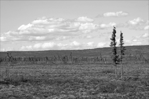
Figure 3. Representative photo of tundra patches in our study area (the Kanuti Lake patch) with a Whimbrel perched on the tallest black spruce in the foreground. Here patches are typically surrounded by a combination of waterbodies, hills, or wooded areas like the black spruce woodland in the distance, with no tundra connectivity between patches to allow family movements (photo: C. Harwood/USFWS).
The breeding phenology of Whimbrels in our study area showed pronounced annual consistency, with arrival, mean nest initiation and mean date of hatch varying by only 5 d across years. Further, mean hatch occurred only about six weeks after the first Whimbrels arrived, suggesting a compressed schedule; no nests hatched (or were scheduled to hatch) after 26 June. Grant (1989) documented annual initiation ranging over periods of 26–31 d for Whimbrels nesting in temperate Shetland, more than twice the longest initiation period that we observed. In 2010 and 2012, in which initiation in our study area occurred over about two weeks, the latest nests (n = 4) all failed, including three that were abandoned. This suggests that late nesting at this site is not generally successful (e.g., Smith et al. 2010), perhaps because this northern latitude and boreal climate impose a shorter window for successful breeding.
Given the spatial and temporal constraints imposed on Whimbrels breeding in our study area, we had hypothesized that predators might more efficiently target nesting Whimbrels here; in turn, these Whimbrels might nest in ways that facilitate cooperative nest and chick defense (i.e., clustered and synchronized nesting). Support for this premise was equivocal. We documented fairly synchronous nesting in 2009 and 2011, but less so in 2010 and 2012; however, we recognize that the compressed breeding schedule here necessarily increases synchrony more so than at sites with longer seasons. Clustered nesting was suggested for Kanuti Lake in 2009, but not for the Everglades. Despite these inconsistent results, nests may still be close enough for neighboring pairs to jointly mob effectively.
Nesting habitat and nest-site selection
Whimbrels nesting in our study area encounter a diverse suite of avian and terrestrial predators that vary in hunting behavior. This diversity of predators could demand potentially conflicting nest protection strategies, such as timely predator detection and nest crypsis. Our hypothesis that Whimbrels here would optimize a tradeoff between nest concealment and view to limit predation was partly supported: nesting on a hummock (thus providing greater view) and greater lateral nest concealment were both shown to be important factors in nest-site selection at the smallest scale. Hummock use has been widely documented in Whimbrels (in Ballantyne & Nol 2011). Our result provides further support that hummocks may be important for early detection of aerial predators. However, Ballantyne & Nol (2011) proposed an alternate hypothesis that hummocky sites melt out earlier, as is true in our study area, and this is advantageous to early nesting species such as Whimbrels. Unlike Skeel (1983), who attributed lateral protrusions of vegetation at nests to protection from prevailing winds, we believe this attribute to be more locally important as camouflage. Our finding of marginal support for nesting areas having greater surface roughness may be further evidence for the importance of habitat complexity (e.g., pattern disruption, increased shadow) in nest concealment, as also suggested by Skeel (1983). Several other measures of complexity, however, were not shown to be important predictors of habitat use in our study.
We found little support for predictors of nest-site selection at larger spatial scales. This could be explained in several ways. For example, the 50-m ‘territorial’ radius may have been too small to reveal differences between nest and random point locations, given the relative homogeneity of the habitat.
Other studies (Pirie 2008, Ballantyne & Nol 2011) used larger distances (250 and 150 m, respectively) in their nest-site selection investigations. Another factor could have been the timing of our habitat measurements. While collecting habitat measurements after nests have hatched is a common practice, this delay risks missing early habitat distinctions evident to Whimbrels during nest-prospecting, such as patterns of snow melt and preleaf-out vegetative cover.
Alternatively, some of our seemingly equivocal habitat selection results may actually be representative for Whimbrels breeding within tundra patches in boreal forest. These birds may simply be generalists at certain scales when selecting a nest site within a suitable patch of habitat. The species has a demonstrated flexibility in nesting habitat selection at the landscape or patch scale throughout other parts of its range. Whimbrels outside of Alaska have been documented nesting in multiple habitat types including hummock-bog, sedge meadow, heathland tundra, riverplain, and even mountain birch forest (Skeel 1983, Pulliainen & Saari 1993, Katrínardóttir et al. 2015). We observed Whimbrels using sites with varying levels of surface roughness, cover heterogeneity, and woody vegetation near the nest, but these may represent minor variations within the nest-site selection repertoire of this widely distributed species.
Table 3. Logistic regression model selection results used to predict Whimbrel nest-site selection (nest vs. random point within the territory) as a function of four habitat variables measured within a scale of 0–400 m from the nest or random point, Kanuti Lake and Everglades study areas, Kanuti National Wildlife Refuge, Alaska, 2011–2012. Models are ordered by Akaike’s Information Criterion, corrected for small sample size (AICc). K is the number of parameters, ∆AICc is the AIC difference from the top model, and –LL is the negative log-likelihood, a measure of deviance. The four variables considered were distances to nearest low shrub (Low), medium shrub (Medium), tall shrub (Tall), and tree (Tree). The 16 candidate models were ultimately averaged. No models received greater support than the null model, so model weights were not calculated/ shown.
Model
K
∆AICc1
–LL
Null
1
0.00
54.07
Low
2
1.63
53.83
Medium
2
1.66
53.84
Tall
2
1.98
54.00
Tree
2
2.10
54.06
Med + Low
3
3.10
53.48
Tree + Medium
3
3.61
53.74
Tall + Low
3
3.69
53.77
Tree + Low
3
3.80
53.83
Tall + Medium
3
3.81
53.83
Tree + Tall
3
4.07
53.96
Tree + Medium + Low
4
5.13
53.38
Tall + Medium + Low
4
5.33
53.48
Tree + Tall + Medium
4
5.74
53.69
Tree + Tall + Low
4
5.88
53.76
Tree + Tall + Medium + Low
5
7.39
53.37
1AICc value of the top model is 110.18.
Table4.Logistic regression model selection results used to predict Whimbrel nest-site selection (nest vs. random point within the territory) as a function of four habitat variables measured at a scale of 0–10 m from the nest orrandom point, Kanuti Lake and Everglades study areas, Kanuti National Wildlife Refuge, Alaska, 2011–2012. Models are ordered by Akaike’s Information Criterion, corrected for small sample size (AICc). K is the number of parameters, ∆AICcis the AIC difference from the top model, and –LL is the negative log-likelihood, a measure of deviance. The four variables tested included measures of (1) surface roughness (AdjHt) and (2) relative height of nest to surrounding surfaces (RelCup), (3) cover hetero- geneity (Cover), and (4) number of medium or tall shrubs(Shrub). The 16 candidate models were ultimately averaged. Only the model with ‘AdjHt’ variable received even marginal support over the null model; thus, model weights were not calculated/shown.
Model
K
∆AICc1
–LL
AdjHt
2
0.00
52.62
Null
1
0.79
54.07
RelCup + AdjHt
3
1.95
52.51
Shrub + AdjHt
3
2.16
52.62
Cover + AdjHt
3
2.16
52.62
RelCup
2
2.59
53.91
Cover
2
2.78
54.01
Shrub
2
2.89
54.06
Shrub + RelCup + AdjHt
4
4.17
52.51
RelCup + Cover + AdjHt
4
4.18
52.51
Shrub + Cover + AdjHt
4
4.38
52.62
RelCup + Cover
3
4.65
53.86
Shrub + RelCup
3
4.75
53.91
Shrub + Cover
3
4.94
54.01
Shrub + RelCup + Cover + AdjHt
5
6.45
52.51
Shrub + RelCup + Cover
4
6.87
53.86
1AICcvalue of the top model is 109.39.
Nest survival
Ultimately we found little support for our hypotheses that nesting earlier, nearer to conspecifics, and with fewer large obstacles near the nest were important factors for nest survival. However, we did find a very strong site effect between our two main study areas; DSR was consistently higher at the Everglades than at Kanuti Lake.
Other studies have documented that Whimbrels nesting in different habitat types may experience different levels of nest success (Skeel 1983, Pulliainen & Saari 1993, Katrínardóttir et al. 2015). Although we characterized Whimbrel territories similarly at the two sites, we did note coarse differences not necessarily captured by our assessments; for example, we noted a dominance of string bogs at Everglades, but less so at Kanuti Lake. Further, the most recent wildfires at Everglades and Kanuti Lake occurred in 1977 and 2005, respectively. Burn perimeters and unburned inclusions are evident at both sites, with Whimbrels nesting among them; however, vegetation recovery at Everglades was more advanced (e.g., no mineral soil visible, less burned duff, more lichen). Whether the likely wetter and less recently burned habitats of the Everglades impart advantages in nest survival is unknown.
Contrary to our expectations, the presence of nearby trees and large shrubs did not influence nest site selection or impair nest survival. Whimbrels breeding in our study area appeared to tolerate, and to some extent even exploit (e.g., as sentry perches; Fig. 3), scattered black spruce in the tundra. Indeed, the three major breeding concentrations (‘east’ and ‘west’ Kanuti Lake, Everglades) partly surround conspicuous, isolated black spruce groves (ca. 0.01–0.03 km²) within the tundra patches, with nests as close as 10 m to the groves. Scattered medium and tall shrubs also were not strongly avoided. While we do not know what threshold of tree and shrub cover will be tolerated, we have observed Whimbrel occupying much shrubbier sites elsewhere in the species’ range (e.g., Donnelly Training Area, Alaska; CMH unpubl. data). However, for Whimbrels attempting to breed in small tundra patches like those at Kanuti NWR, increased woody vegetation within the patch and encroachment of trees and shrubs inward from the edge could jeopardize the persistence of these patches as open habitats. The increases in shrub and tree cover recently documented at Churchill, Manitoba, Canada, have likely contributed to a decline of Whimbrels there (Ballantyne & Nol 2015), and similar habitat changes have also been predicted for Alaska under a warming climate scenario (Lloyd 2005, Tape et al. 2006).
Table 5. Logistic regression model selection results used to predict Whimbrel nest-site selection (nest vs. random point within the territory) as a function of four habitat variables measured at a scale of 0–1 m from the nest or random point, Kanuti Lake and Everglades study areas, Kanuti National Wildlife Refuge, Alaska, 2011–2012. Models are ordered by Akaike’s Information Criterion, corrected for small sample size (AICc). K is the number of parameters, ∆AICc is the AIC difference from the top model, wi is AICc weight, and –LL is the negative log-likelihood, a measure of deviance. The four variables tested included (1) whether nest was on a hummock (Hummock), (2) nest concealment (Conceal), (3) cover heterogeneity (Cover), and (4) an alternate measure of roughness (Rough). The candidate models contributing to the cumulative AICc were ultimately averaged. Model weight for model named ‘Cover’ (ranked lower than Null) was not calculated.
Model
K
∆AICc1
wi
–LL
Hummock + Conceal + Cover
4
0
0.35
38.1
Hummock + Conceal + Cover + Rough
5
0.09
0.33
37
Hummock + Conceal
3
1.68
0.15
40.06
Hummock + Conceal + Rough
4
2.65
0.09
39.42
Hummock
2
5.55
0.02
43.07
Hummock + Cover + Rough
4
5.89
0.02
41.05
Hummock + Rough
3
6.13
0.02
42.28
Hummock + Cover
3
6.22
0.02
42.32
Conceal + Cover + Rough
4
8.77
0
42.49
Conceal + Rough
3
13.11
0
45.77
Conceal + Cover
3
16.4
0
47.41
Cover + Rough
3
16.48
0
47.45
Rough
2
18
0
49.3
Conceal
2
18.4
0
49.5
Null
1
25.43
0
54.07
Cover
2
26.28
–
53.43
1AICc value of the top model is 84.75.
Boreal-nesting Whimbrels and wildfire
The active fire history that regularly and dynamically affects our area (e.g., 27% of Kanuti NWR burned in 2004–2005; USFWS 2008) has not been documented in other areas where Whimbrels have been studied. Although wildfires are frequent within the greater Hudson Bay Lowlands (Brook 2006), Whimbrels breeding near Churchill appear to use areas just outside this fire regime (Fig. 2.2 in Ballantyne 2009), perhaps a result of the proximity of these areas to the maritime influence of Hudson Bay. In general, we lack a perspective on how Whimbrels respond to major stochastic events that have impacted their landscapes (but see Katrínardóttir et al. 2015). During our study, we observed annual fluctuations in numbers and distribution, but we do not know how Whimbrels in the Everglades and Kanuti Lake areas responded immediately after wildfires in 1977 and 2005, respectively.
Table 6. Model selection results for analysis testing potential factors of daily survival rate (DSR) for Whimbrel nests at Kanuti Lake and Everglades study areas, Kanuti National Wildlife Refuge, Alaska, 2009–2012. Models are ordered by Akaike’s Information Criterion, corrected for small sample size (AICc). K is the number of parameters, ∆AICc is the AIC difference from the top model, wiis AICc weight. The ten models tested DSR of nests (1) ‘Constant’ through season; and then varying (2) through‘Season’, (3) by‘Year’, (4) by study area (Site), (5) by Site*Year interaction, (6) by age of nest (NestAge), (7) by age of nest when found (AgeFound), (8) by nearest inter-nest distance (InterDist), (9) by number of nearby large shrubs (Shrub), and (10) by presence of nearby trees. Model weights were not calculated for unsupported models (i.e., ranked lower than the constant model).
Model
K
∆AICc
1
wi
Deviance
Site
2
0
0.79
162.01
Site*Year
6
3.44
0.14
157.37
Season
2
5.46
0.05
167.47
AgeFound
2
9.08
0.01
171.09
Constant
1
9.28
0.01
173.29
NestAge
2
9.6
–
171.6
Year
4
9.97
–
167.95
Tree
2
10.19
–
172.2
Shrub
2
10.98
–
172.99
InterDist
2
11.16
–
173.16
1AICc value of the top model is 84.75.
Within the already dynamic landscape of boreal Alaska, we may be witnessing additional effects on habitats from the projected increase in landscape flammability across the boreal forest during the coming century (Rupp & Springsteen 2009, Johnstone et al. 2011). The possible amplification of the area’s historical wildfire regime by a warming climate may pose a major threat to not only forested habitats (e.g., conversion of spruce to deciduous), but could result in the loss or modification (e.g., increased shrubs) of boreal tundra patches suitable for Whimbrel breeding. Studies of predicted changes in the boreal biome have focused on forests proper, and studies of tundra fires have targeted areas beyond the treeline (Higuera et al. 2011), not tundra patches within the boreal. Studies like ours can serve as baselines for monitoring these scattered tundra patches, and the persistence of Whimbrels therein. Further, replication of our study in other areas offers an approach to improve inference from local studies like ours (‘metareplication’; Johnson 2002). Our research clearly shows the benefit of conducting regular surveys of historical Whimbrel breeding areas accessible within the boreal forest to document local persistence of the species and to characterize its habitat. We especially urge a timely survey of a recently burned breeding areas to asses any changes to habitats and responses by the local Whimbrel population to wildfire effects. In time we can begin to better assess the vulnerability of Whimbrels and their habitats in a rapidly changing boreal biome.
ACKNOWLEDGEMENTS
We thank the staff of Kanuti NWR for their generous and persistent support of this project. We especially thank the following field assistants: L. Smithwick, P. Valle, L. Tibbitts, N. Senner, S. Warnock, D. Kaleta, E. Garrett, R. Dugan, D. Smith, J. McLaughlin, and N. Wepking. This paper benefited from reviews by J. Perz, D. Ruthrauff, P. Smith, and D. Verbyla. A.-M. Benson and C. Handel provided valuable analytical assistance. This study was performed under the auspices of U.S. Fish and Wildlife Service, Region 7, Institutional Animal Care and Use Committee (IACUC) protocol #2010007. Unpublished reports cited in this paper are available at Alaska Resources Library and Information Services, www.arlis.org. Any use of trade, product, or firm names in this publication is for descriptive purposes only and does not imply endorsement by the U.S. Government.
REFERENCES
Alaska Climate Research Center. 2013. May 2013 statewide summary. University of Alaska Fairbanks, Fairbanks, Alaska. Accessed 21 Oct 2015 at: http://climate.gi.alaska.edu/ Summary/Statewide/2013/May.
American Ornithologists’ Union (AOU). 1998. Check-list erican birds, 7th ed. American Ornithologists’ Union, Washington, D.C.
Andren, H. & P. Angelstam. 1988. Elevated predation rates as an edge effect in habitat islands: experimental evidence. Ecology 69: 544–547.
Andres, B.A., P.A. Smith, R.I.G. Morrison, C.L. Gratto– Trevor, S.C. Brown & C.A. Friis. 2012. Population estimates of North American shorebirds, 2012. Wader Study Group Bulletin 119: 178–194.
Arnold. T.W. 2010. Uninformative parameters and model selection using Akaike’s Information Criterion. Journal of Wildlife Management 74: 1175–1178.
Bailey, J. & F.R. Thompson. 2007. Multiscale nest-site selection by Black-capped Vireos. Journal of Wildlife Man- agement 71: 828–836.
Ballantyne, K. 2009. Whimbrel (Numenius phaeopus) nesting habitat associations, altered distribution & habitat change in Churchill, Manitoba, Canada. MSc thesis, Trent Uni- versity, Peterborough, Ontario.
Ballantyne, K. & E. Nol. 2011. Nesting habitat selection and hatching success of Whimbrels near Churchill, Man- itoba, Canada. Waterbirds 34: 151–159.
Ballantyne, K. & E. Nol. 2015. Localized habitat change near Churchill, Manitoba and the decline of nesting Whimbrels (Numenius phaeopus). Polar Biology 38: 529–537.
Blevins, E. & K. With. 2011. Landscape context matters: local habitat and landscape effects on the abundance and patch occupancy of collared lizards in managed grasslands. Landscape Ecology 26: 837–850.
Booth, D.T., S.E. Cox & R.D. Berryman. 2006. Point sampling digital imagery with ‘SamplePoint.’ Environmental Monitoring and Assessment 123: 97–108.
Brook, R. 2006. Forest and tundra fires in the Hudson Bay Lowlands of Manitoba. Pp. 365–378 in: Climate change: linking traditional and scientific knowledge (J. Oakes & R. Riewe, Eds.). Aboriginal Issues Press, University of Man- itoba, Winnipeg, Manitoba.
Brown, S.C., H.R. Gates, J.R. Liebezeit, P.A. Smith, B.L. Hill & R.B. Lanctot. 2014. Arctic Shorebird Demographics Network breeding camp protocol, version 5, April 2014. Unpublished paper, U.S. Fish and Wildlife Service and Manomet Center for Conservation Sciences. Accessed 21 Oct 2015 at: https://www.manomet.org/sites/default/files/ publications_and_tools/ASDN_Protocol_V5_20Apr2014.pdf.
Burnham, K.P. & D.R. Anderson. 2002. Model selection and multimodel inference: a practical information-theoretic approach. Second edition. Springer-Verlag, New York.
Cramp, S. & K.E.L. Simmons (Eds). 1983. Handbook of the birds of Europe, the Middle East and North Africa. The birds of the western Palearctic: vol. III: waders to gulls. Oxford University Press, Oxford, UK.
Engelmoer, M. & C.S. Roselaar. 1998. Geographical variation in waders. Kluwer Academic Publishers, Dordrecht, The Netherlands.
Fleishman, E., C. Ray, P. Sjögren-Gulve, C.L. Boggs & D.D. Murphy. 2002. Assessing the roles of patch quality, area, and isolation in predicting metapopulation dynamics. Conservation Biology 16: 706–716.
Fortin, M.-J. & M.R. Dale. 2005. Spatial analysis: a guide for ecologists. Cambridge University Press, New York.
Frolking, S., J. Talbot, M.C. Jones, C.C. Treat, J.B. Kauffman, E.-S. Tuittila & N. Roulet. 2011. Peatlands in the Earth’s 21st century climate system. Environmental Reviews 19: 371–396.
Gibson, D.D. 2011. Nesting shorebirds and landbirds of interior Alaska. Contract Order No. G10PX02562, AVESALASKA, Ester, AK. [Available through Alaska Resources Library and Information Services,www.arlis.org]
Gómez-Serrano, M.Á. & P. López-López. 2014. Nest site selection by Kentish Plover suggests a trade-off between nest-crypsis and predator detection strategies. PLoS ONE 9(9): e107121. doi:10.1371/journal.pone.0107121.
Götmark, F., D. Blomqvist, O.C. Johansson & J. Bergkvist. 1995. Nest site selection: a trade-off between concealment and view of the surroundings? Journal of Avian Biology 26: 305–312.
Gotthardt, T., S. Pyare, F. Huettmann, K. Walton, M. Spathelf, K. Nesvacil, A. Baltensperger, G. Humphries & T. Fields. 2013. Alaska Gap Analysis Project terrestrial vertebrate species atlas. The Alaska Gap Analysis Project, University of Alaska, Anchorage. Accessed 10 Feb 2013 at:http://akgap.uaa.alaska.edu/publications.
Grant, M.C. 1989. The breeding ecology of Whimbrel (Numenius phaeopus) in Shetland: with particular reference to the effects of agricultural improvement of heathland nesting habitats. PhD thesis, Durham University, Durham, UK.
Grosse, G., J. Harden, M. Turetsky, A.D. McGuire, P. Camill, C. Tarnocai, S. Frolking, E.A.G. Schuur, T. Jor- genson, S. Marchenko, V. Romanovsky, K.P. Wickland,
N. French, M. Waldrop, L. Bourgeau-Chavez & R.G. Striegl. 2011. Vulnerability of high-latitude soil organic carbon in North America to disturbance. Journal of Geo- physical Research 116: G00K06. doi:10.1029/2010JG001507.
Grueber, C.E., S. Nakagawa, R.J. Laws & I.G. Jamieson. 2011. Multimodel inference in ecology and evolution: challenges and solutions. Journal of Evolutionary Biology 24: 699–711.
Hartman, C.A. & L.W. Oring. 2006. An inexpensive method for remotely monitoring nest activity. Journal of Field Ornithology 77: 418–424.
Higuera, P.E., M.L. Chipman, J.L. Barnes, M.A. Urban &
F.S. Hu. 2011. Variability of tundra fire regimes in arctic Alaska: millennial-scale patterns and ecological implications. Ecological Applications 21: 3211–3226.
Jehl, Jr. J.R. 1971. Patterns of hatching success in subarctic birds. Ecology 52: 169–173.
Johnson, D.H. 2002. The importance of replication in wildlife research. Journal of Wildlife Management 66: 919–932.
Johnstone, J., T.S. Rupp, M. Olson & D. Verbyla. 2011. Modeling impacts of fire severity on successional trajectories fire behavior in Alaskan boreal forests. Landscape Ecology 26: 487–500.
Jones, J. & R.J. Robertson. 2001. Territory and nest-site selection of Cerulean Warblers in eastern Ontario. Auk 118: 727–735.
Jorgenson, T.M. & D. Meidinger. 2015. The Alaska-Yukon region of the circumboreal vegetation map: final report. CAFF strategies series report. Conservation of Arctic Flora and Fauna, Akureyri, Iceland.
Kasischke, E.S., T.S. Rupp & D.L. Verbyla. 2006. Fire trends in the Alaskan boreal forest. Pp. 285–301 in: Alaska’s changing boreal forest (F.S. Chapin III, M. Oswood, K. Van Cleve, L.A. Viereck & D. Verbyla, Eds.). Oxford Uni- versity Press, New York.
Kasischke, E.S. & M.R. Turetsky. 2006. Recent changes in the fire regime across the North American boreal region— spatial and temporal patterns of burning across Canada and Alaska. Geophysical Research Letters 33: L09703. doi:10.1029/2006GL025677.
Kasischke, E.S., D.L. Verbyla, T.S. Rupp, A.D. McGuire,
K.A. Murphy, R. Jandt, J.L. Barnes, E.E. Hoy, P.A. Duffy, M. Calef & M.R. Turetsky. 2010. Alaska’s changing fire regime—implications for the vulnerability of its boreal forests. Canadian Journal of Forest Research 40: 1313–1324.
Katrínardóttir, B. 2012. The importance of Icelandic riverplains as breeding habitats for Whimbrels Numenius phaeopus. MSc thesis, University of Iceland, Reykjavik.
Katrínardóttir, B., J.A. Alves, H. Sigurjónsdóttir, P. Her- steinsson & T.G. Gunnarsson. 2015. The effects of habitat type and volcanic eruptions on the breeding demography of Icelandic Whimbrels Numenius phaeopus. PLoS ONE 10(7): e0131395. doi:10.1371/journal.pone.0131395.
Lele, S.R., J.L. Keim & P. Solymos. 2014. Package ‘Resource Selection: Resource Selection (Probability) Functions for Use-Availability Data,’ R Package version 0.2-4. Accessed 12 Aug 2014 at: http://cran.r-project.org/package=Resource- Selection.
Liebezeit, J.R., P.A. Smith, R.B. Lanctot, H. Schekkerman,
I. Tulp, S.J. Kendall, D.M. Tracy, R.J. Rodrigues, H. Meltofte, J.A. Robinson, C. Gratto-Trevor, B.J. McCaffery,
J. Morse & S.W. Zack. 2007. Assessing the development of shorebird eggs using the flotation method: species- specific and generalized regression models. Condor 109: 32–47.
Lloyd, A.H. 2005. Ecological histories from Alaskan tree lines provide insight into future change. Ecology 86: 1687– 1695.
Marks, J.S., T.L. Tibbitts, R.E. Gill, Jr. & B.J. McCaffery. 2002. Bristle-thighed Curlew (Numenius tahitiensis). In: The Birds of North America Online (A. Poole, Ed.). Cornell Lab of Ornithology, Ithaca. Accessed at: http://bna.birds.cor- nell.edu/bna/species/705, doi:10.2173/bna.705.
Mazerolle, M.J. & M.-A. Villard. 1999. Patch characteristics and landscape context as predictors of species presence and abundance: a review. Ecoscience 6: 117–124.
McCaffery, B.J. 1996. The status of Alaska’s large shorebirds: a review and an example. International Wader Studies 8: 28–32.
National Wetlands Working Group. 1997. The Canadian wetland classification system. Second Edition (B.G. Warner
& C.D.A. Rubec, Eds.). Report 0662258576. Wetlands Research Centre, University of Waterloo, Waterloo, Ontario. Accessed 28 Oct 2014 at: http://www.gret-perg.ulaval.ca/file admin/fichiers/fichiersGRET/pdf/Doc_generale/Wetlands.pdf.
Neipert, E., M. Cameron, J. Dacey & J. Haddix. 2014. Monitoring of subalpine Whimbrels on Donnelly Training Area, Fort Wainwright, AK. Unpublished resource report. Delta Junction, Alaska, USA. [Available through Alaska Resources Library and Information Services, www.arlis.org]
Nol, E., M.S. Blanken & L. Flynn. 1997. Sources of variation in clutch size, egg size and clutch completion dates of Semipalmated Plovers in Churchill, Manitoba. Condor 99: 389–396.
Payette, S., M.-J. Fortin & I. Gamache. 2001. The subarctic forest-tundra: the structure of a biome in a changing climate. BioScience 51: 709–718.
Pirie, L.D. 2008. Identifying and modeling Whimbrel Numenius phaeopus breeding habitat in the outer Mackenzie Delta, Northwest Territories. MSc thesis, Carleton University, Ottowa, Canada.
Pirie, L.D., C.M. Francis & V.H. Johnston. 2009. Evaluating the potential impact of a gas pipeline on Whimbrel breeding habitat in the outer Mackenzie Delta, Northwest Territories. Avian Conservation & Ecology-Écologie et con- servation des oiseaux 4: 2.
Pulliainen, E. & L. Saari. 1993. Breeding biology of the Whimbrel Numenius phaeopus in eastern Finnish Lapland. Ornis Fennica 70: 110–116.
R Development Core Team. 2014. R: A language and envi- ronment for statistical computing. R Foundation for Statistical Computing, Vienna, Austria. Accessed 31 Aug 2015 at: http://www.R-project.org.
Riordan, B., D. Verbyla & A.D. McGuire. 2006. Shrinking ponds in subarctic Alaska based on 1950–2002 remotely sensed images. Journal of Geophysical Research 111: G04002. doi:10.1029/2005JG000150.
Roach, J.K. 2011. Lake area change in Alaskan National Wildlife Refuges: magnitude, mechanisms, and heterogeneity. PhD thesis, University of Alaska Fairbanks, Fairbanks, Alaska, USA.
Rodrigues, R. 1994. Microhabitat variables influencing nest- site selection by tundra birds. Ecological Applications 4: 110–116.
Rotella, J. 2015. Nest survival models. Chapter 17 in: Program MARK: a gentle introduction (E. Cooch & G. White, Eds.). Accessed 25 July 2015: http://www.phidot.org/soft- ware/mark/docs/book.
Rupp, T.S. & A. Springsteen. 2009. Summary report for Kanuti National Wildlife Refuge: projected vegetation and fire regime response to future climate change in Alaska. Unpublished report, SNAP (Scenarios Network Planning for Alaska & Arctic Planning), University of Alasksa Fair- banks. [Available through Alaska Resources Library and Information Services, www.arlis.org]
Sinclair, P.H., W.A. Nixon, C.D. Eckert & N.L. Hughes. 2003. Birds of the Yukon Territory. UBC Press, Vancouver, British Columbia, Canada.
Skeel, M.A. 1983. Nesting success, density, philopatry, and nest-site selection of the Whimbrel (Numenius phaeopus) in different habitats. Canadian Journal of Zoology 61: 218–225.
Skeel, M.A. & E.P. Mallory. 1996. Whimbrel (Numenius phaeopus). In: The Birds of North America, No. 219 (A. Poole & F. Gill, Eds.). The Birds of North America, Inc. Philadelphia, PA.
Smith, P.A., H.G. Gilchrist, M.R. Forbes, J.-L. Martin & K. Allard. 2010. Inter-annual variation in the breeding chronology of arctic shorebirds: effects of weather, snow melt and predators. Journal of Avian Biology 41: 292–304.
Tape, K., M. Sturm & C. Racine. 2006. The evidence for shrub expansion in northern Alaska and the Pan-Arctic. Global Change Biology 12: 686–702.
U.S. Fish and Wildlife Service (USFWS). 2008. Revised comprehensive conservation plan for the Kanuti National Wildlife Refuge. U.S. Fish and Wildlife Service, Anchorage, Alaska. [Available through Alaska Resources Library and Information Services, www.arlis.org or at: http://www.fws.gov/uploadedFiles/Region_7/NWRS/Zone_1/Kanuti/PDF/Ka nuti_ccp.pdf]
van der Vliet, R.E., E. Schuller & M.J. Wassen. 2008. Avian predators in a meadow landscape: consequences of their occurrence for breeding open-area birds. Journal of Avian Biology 39: 523–529.
Viereck, L.A., C.T. Dyrness, A.R. Batten & K.J. Wenzlick. 1992. The Alaska vegetation classification. General Technical Report PNW–GTR–286. U.S. Department of Agriculture, Forest Service, Pacific Northwest Research Station, Portland, OR. [Available through Alaska Resources Library and Information Services, www.arlis.org or at: http://www.fws. gov/refuge/Kanuti/what_we_do/planning.html]
Wells, J.V. & P. Blancher. 2011. Global role for sustaining bird populations. Chapter 2 in: Boreal birds of North America (J.V. Wells, Ed.). Studies in Avian Biology 41: 7– 22.
White, G.C. & K.P. Burnham. 1999. Program MARK: survival estimation from populations of marked animals. Bird Study 46: S120–S139.
With, K.A. & A.W. King. 2001. Analysis of landscape sources and sinks: the effect of spatial patter on avian demography. Biological Conservation 100: 75–88.